Quantifying trend days
In my first blog post I want to show you a way to mathematically define trend days. Trend days are easy to spot (in hindsight) with the naked eye but you probably don't want to weed through 10 years of intraday data manually. Defining a simple "trendiness" measurement can help answering a lot of questions programmatically:
- Is there a typical behaviour before or after a trend day?
- Are trend days distributed evenly among the weekdays?
- Do trend days cluster or are they evenly distributed over time?
- How trendy is a market?
- Etc.
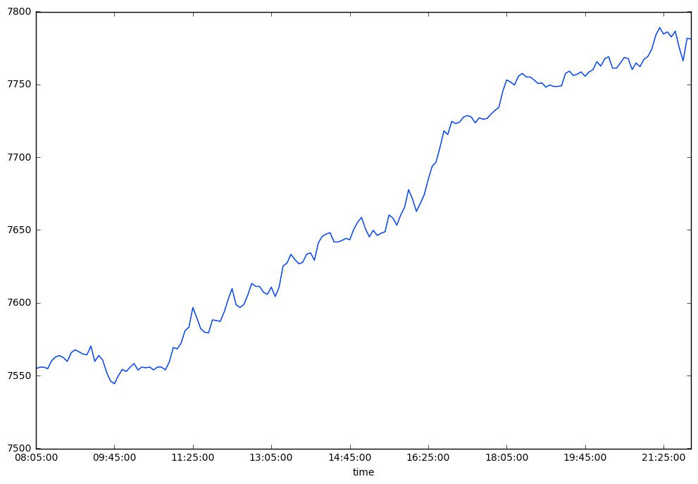
Have a look at last Wednesday's DAX chart:

DAX 5 Minute Chart, 14.3.18
The blue line shows the intraday closing price of DAX. The green line represents the trend. It's a linear regression of the closing price on the index (1-168). If you don't know what linear regression is, you can think of it as the best-fitting straight line through all the data points. The red bars show the deviation of the actual closing price and the regression line, in statistical terms these are called residuals.
These deviations are exactly what we will be looking at. A trend day will have smaller deviations while a choppy day's deviations will be larger. We can use the coefficient of determination (or simply: R2) to measure this deviation. The R2 will always range between 0 and 1. An R2 of 1 means that there's a perfect trend (every closing price is exactly on the green line) while an R2 of 0 means that there is no underlying trend.
We can easily calculate this measure in python with the help of pandas and statsmodels. Assuming you have loaded the data in a pandas dataframe like this:
We then write a function, apply it row-wise to the dataframe and save it in a new column called 'rsquared'.
import statsmodels.api as sm

(...)

def rsquared(row):
    X = sm.add_constant(range(0, len(row.values)))
    y = row.values
    result = sm.OLS(y, X).fit()
    return result.rsquared

df.loc[:, 'rsquared'] = df.apply(rsquared,axis=1)
Now that we have a trend measure for each day of the past 10 years let's have a look at the distribution of the R2 values. Most of the days have no trend at all:
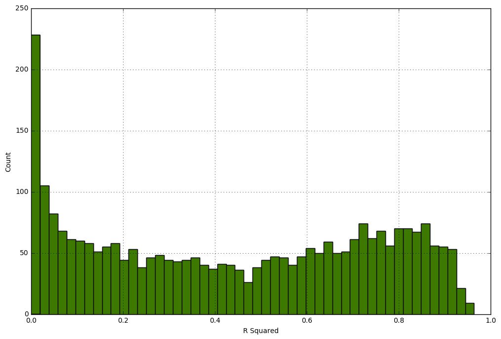
Distribution of R-Squared Values
We can also look at the most (R2 = 0.96) and the least (R2 = 0) "trendy" day of the data set:
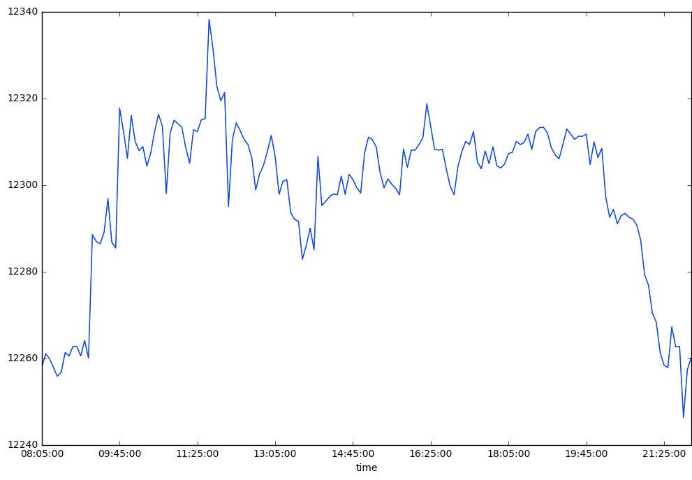
23.11.2007 vs. 26.7.2017
In a follow up post I'll try to answer some of the questions mentioned in the beginning of this post. If you have any question let me know in the comments below or hit me up on Twitter.